Laplace distribution
| Probability density function |
|
| Cumulative distribution function |
|
| Parameters |  location (real) location (real) scale (real) scale (real) |
|---|---|
| Support |  |
 |
|
| CDF | see text |
| Mean | |
| Median | |
| Mode | |
| Variance |  |
| Skewness |  |
| Ex. kurtosis |  |
| Entropy |  |
| MGF |  for for  |
| CF |  |
In probability theory and statistics, the Laplace distribution is a continuous probability distribution named after Pierre-Simon Laplace. It is also sometimes called the double exponential distribution, because it can be thought of as two exponential distributions (with an additional location parameter) spliced together back-to-back, but the term double exponential distribution is also sometimes used to refer to the Gumbel distribution. The difference between two independent identically distributed exponential random variables is governed by a Laplace distribution, as is a Brownian motion evaluated at an exponentially distributed random time. Increments of Laplace motion or a variance gamma process evaluated over the time scale also have a Laplace distribution.
Contents |
Characterization
Probability density function
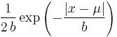
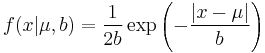
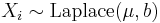
A random variable has a Laplace(μ, b) distribution if its probability density function is
![= \frac{1}{2b}
\left\{\begin{matrix}
\exp \left( -\frac{\mu-x}{b} \right) & \mbox{if }x < \mu
\\[8pt]
\exp \left( -\frac{x-\mu}{b} \right) & \mbox{if }x \geq \mu
\end{matrix}\right.](/2012-wikipedia_en_all_nopic_01_2012/I/ce4d439591049ac1d53672d9035bf685.png)
Here, μ is a location parameter and b > 0 is a scale parameter. If μ = 0 and b = 1, the positive half-line is exactly an exponential distribution scaled by 1/2.
The probability density function of the Laplace distribution is also reminiscent of the normal distribution; however, whereas the normal distribution is expressed in terms of the squared difference from the mean μ, the Laplace density is expressed in terms of the absolute difference from the mean. Consequently the Laplace distribution has fatter tails than the normal distribution.
Cumulative distribution function
The Laplace distribution is easy to integrate (if one distinguishes two symmetric cases) due to the use of the absolute value function. Its cumulative distribution function is as follows:
 |
 |
![= \left\{\begin{matrix}
&\frac12 \exp \left( \frac{x-\mu}{b} \right) & \mbox{if }x < \mu
\\[8pt]
1-\!\!\!\!&\frac12 \exp \left( -\frac{x-\mu}{b} \right) & \mbox{if }x \geq \mu
\end{matrix}\right.](/2012-wikipedia_en_all_nopic_01_2012/I/668a7fb956fa46baea2606536f2f4dc8.png) |
|
![=0.5\,[1 %2B \sgn(x-\mu)\,(1-\exp(-|x-\mu|/b))].](/2012-wikipedia_en_all_nopic_01_2012/I/390e84f8a1ff892a4aa985000a994453.png) |
The inverse cumulative distribution function is given by

Generating random variables according to the Laplace distribution
Given a random variable U drawn from the uniform distribution in the interval (-1/2, 1/2], the random variable

has a Laplace distribution with parameters μ and b. This follows from the inverse cumulative distribution function given above.
A Laplace(0, b) variate can also be generated as the difference of two i.i.d. Exponential(1/b) random variables. Equivalently, a Laplace(0, 1) random variable can be generated as the logarithm of the ratio of two iid uniform random variables.
Parameter estimation
Given N independent and identically distributed samples x1, x2, ..., xN, the maximum likelihood estimator  of
of  is the sample median,[1] and the maximum likelihood estimator of b is
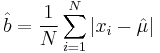
(revealing a link between the Laplace distribution and least absolute deviations).
Moments
![\mu_r' = \bigg({\frac{1}{2}}\bigg) \sum_{k=0}^r \bigg[{\frac{r!}{k! (r-k)!}} b^k \mu^{(r-k)} k! \{1 %2B (-1)^k\}\bigg]](/2012-wikipedia_en_all_nopic_01_2012/I/79014853bc474b0a516b0fad86c456df.png)
Related distributions
- If
 then
then 
- If
 then
then  (exponential distribution)
 - If
 and
and  then
then  .
. - If
 then
then 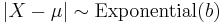
- If then
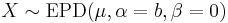 (Exponential power distribution)
 - If
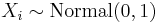 (Normal distribution) for
 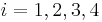 then
then 
- If
 then
then 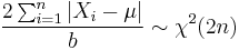 (Chi-squared distribution)
 - If
 and
and  then
then 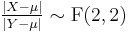 (F-distribution)
 - If
 and
and  (Uniform distribution (continuous)) then
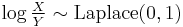
- If
 and
and 
 independent of
  , then
  .
. - If
 and
and  independent of
  , then
  .
. - If
 and
and  independent of
  , then
  .
. - If
 is a geometric stable distribution with
  =2,
=2,  =0 and =0 then
  is a Laplace distribution with
  and b=
- Laplace distribution is the limiting case of Hyperbolic distribution
- If
 with
with  (Rayleigh distribution) then
Relation to the exponential distribution
A Laplace random variable can be represented as the difference of two iid exponential random variables.[2] One way to show this is by using the characteristic function approach. For any set of independent continuous random variables, for any linear combination of those variables, its characteristic function (which uniquely determines the distribution) can be acquired by multiplying the correspond characteristic functions.
Consider two i.i.d random variables  . The characteristic functions for
  are
are  , respectively. On multiplying these characteristic functions (equivalent to the characteristic function of the sum of therandom variables
  ), the result is
  .
.
This is the same as the characteristic function for  , which is
  .
.
Sargan distributions
Sargan distributions are a system of distributions of which the Laplace distribution is a core member. A p'th order Sargan distribution has density[3][4]
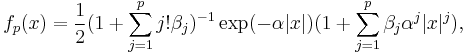
for parameters α > 0, βj ≥ 0. The Laplace distribution results for p=0.
Applications
The Laplacian distribution has been used in speech recognition to model priors on DFT coefficients.
See also
- Log-Laplace distribution
- Cauchy distribution, also called the "Lorentzian distribution" (the Fourier transform of the Laplace)
- Characteristic function (probability theory)
References
- ^ Robert M. Norton (May 1984). "The Double Exponential Distribution: Using Calculus to Find a Maximum Likelihood Estimator". The American Statistician (American Statistical Association) 38 (2): 135–136. doi:10.2307/2683252. JSTOR 2683252.
- ^ The Laplace distribution and generalizations: a revisit with applications to Communications, Economics, Engineering and Finance, Samuel Kotz,Tomasz J. Kozubowski,Krzysztof Podgórski, p.23 (Proposition 2.2.2, Equation 2.2.8). Online here.
- ^ Everitt, B.S. (2002) The Cambridge Dictionary of Statistics, CUP. ISBN 0-521-81099-x
- ^ Johnson, N.L., Kotz S., Balakrishnan, N. (1994) Continuous Univariate Distributions, Wiley. ISBN 0-471-58495-9. p. 60
|
|||||||||||